January 1, 0001
Introduction
The dataset that has been used in the following modeling project is the dataset called ‘USMortality’ that contains mortality rates from the United States by different causes and amongst sex. This dataset contains 40 observations from mortality rates across all ages from the years 2011-2013. Cause of death, sex and rural vs. urban status were recorded among each observation. The variables in this dataset are ‘Status’, ‘Sex’, ‘Cause’, ‘Rate’, and ‘SE’. Status contains whether the individual was of urban or rural status. ‘Sex’ has whether a given individual was male or female. ‘Cause’ contains the particular cause of death of the individual. This variable contains multiple levels of which include, Alzheimers, Cancer, Cerebrovascular diseases, Diabetes, Flu and pneumonia, Heart disease, Lower respiratory, Nephritis, Suicide and Unintentional Injuries. ‘Rate’ is the age-adjusted death rate per 100,000 individuals of the population and ‘SE’ is the standard error of ‘Rate’. A binary variable was added that distinguishes the people of urban status from rural stauts.
Packages Used in Data Analysis
library(dplyr)
library(tidyverse)
library(pROC)
library(sandwich)
library(lmtest)
library(glmnet)
library(plotROC)
Importing ‘USMortality’ Dataset
library(lattice)

head(USMortality)
## Status Sex Cause Rate SE
## 1 Urban Male Heart disease 210.2 0.2
## 2 Rural Male Heart disease 242.7 0.6
## 3 Urban Female Heart disease 132.5 0.2
## 4 Rural Female Heart disease 154.9 0.4
## 53 Urban Male Cancer 195.9 0.2
## 54 Rural Male Cancer 219.3 0.5MANOVA
#eyeball assumptions of multivariate normality
ggplot(USMortality, aes(x = Rate, y = SE)) +
geom_point(alpha = .7) + geom_density_2d() + facet_wrap(~Status)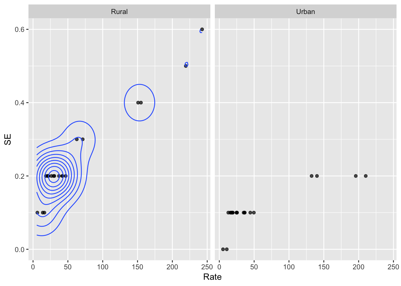
man2 <- manova(cbind(Rate,SE)~Status, data=USMortality)
summary(man2)
## Df Pillai approx F num Df den Df Pr(>F)
## Status 1 0.65536 35.179 2 37 2.763e-09 ***
## Residuals 38
## ---
## Signif. codes: 0 '***' 0.001 '**' 0.01 '*' 0.05 '.' 0.1 ' ' 1summary.aov(man2)## Response Rate :
## Df Sum Sq Mean Sq F value Pr(>F)
## Status 1 1023 1023.1 0.2322 0.6327
## Residuals 38 167467 4407.0
##
## Response SE :
## Df Sum Sq Mean Sq F value Pr(>F)
## Status 1 0.196 0.196000 19.196 8.97e-05 ***
## Residuals 38 0.388 0.010211
## ---
## Signif. codes: 0 '***' 0.001 '**' 0.01 '*' 0.05 '.' 0.1 ' ' 1USMortality%>%group_by(Status)%>%summarize(mean(Rate),mean(SE))## # A tibble: 2 x 3
## Status `mean(Rate)` `mean(SE)`
## <fct> <dbl> <dbl>
## 1 Rural 63.8 0.25
## 2 Urban 53.7 0.11pairwise.t.test(USMortality$Rate,USMortality$Status,
p.adj="none")##
## Pairwise comparisons using t tests with pooled SD
##
## data: USMortality$Rate and USMortality$Status
##
## Rural
## Urban 0.63
##
## P value adjustment method: nonepairwise.t.test(USMortality$SE,USMortality$Status,
p.adj="none")##
## Pairwise comparisons using t tests with pooled SD
##
## data: USMortality$SE and USMortality$Status
##
## Rural
## Urban 9e-05
##
## P value adjustment method: noneUsing MANOVA to determine whether ‘Rate’ or ‘SE’ differ amongst ‘Status’.
H0 : ‘Rate’ and ‘SE’ remain the same by ‘Status’
HA : ‘Rate’ and ‘SE’ differ by ‘Status’
Adjusted alpha by Bonferroni Method: .05/5 = .01
The assumptions of a MANOVA, are random samples and independent observations. This dataset is representative of the Department of Health and Human Services, therefore there is not a definite way for me to determine if these observations were recorded randomly. More assumptions of MANOVA is multivate normality, no extreme multivariate outliers and no multicollinearity of which will be discussed in later paragraphs.
A multivariate analysis of variance (MANOVA) was performed in order to dertermine whether ‘Rate’ or ’SE differed across the statuses rural and urban. Upon examining the plot rural, there were no obvious differences in multivariate normality. Although, the plot for urban status, multivariate normality was not met. When conducting the MANOVA, significant differences were observed amongst the two different statuses.
Different univariate analyses of variance (ANOVAs) were carried out for each dependent variable and to control for Type 1 errors, the Bonferroni method was applied. One MANOVA, two ANOVAs, and two pairwise t-tests which means that our alpha level was adjusted by 5. The univariate ANOVAs also revealed significance with the adjusted Bonferroni alpha level of 0.01. In order to determine which status differed significantly, post-hoc t-tests were conducted. It was revealed that individuals of urban status differed significantly in terms of rate and SE from those of a rural status. Even with the new adjusted alpha level there is still significance among individuals of an urban status.
Randomization Test
urbans <- c(210.2, 132.5, 195.9, 140.2,44.5, 36.5,49.6, 24.7, 36.1,34.9,19.4,25.5,24.9,17.1,17.7,12.9,19.2,5.3,15.7,10.7)

rurals <-c(242.7,154.9,219.3,150.8,62.8,46.9,71.3,37.2,42.2,42.2,21.8,30.6,29.5,21.8,20.8,16.3,26.3,6.2,18.3,13.9)

data1 <-data.frame(Status=c(rep("rurals",20), rep("urbans",20)), Rate=c(rurals,urbans))

ggplot(data1,aes(Rate,fill=Status))+geom_histogram(bins=6.5)+facet_wrap(~Status,ncol=2) +theme_minimal() + ggtitle("Rates Among Rural vs. Urban Status")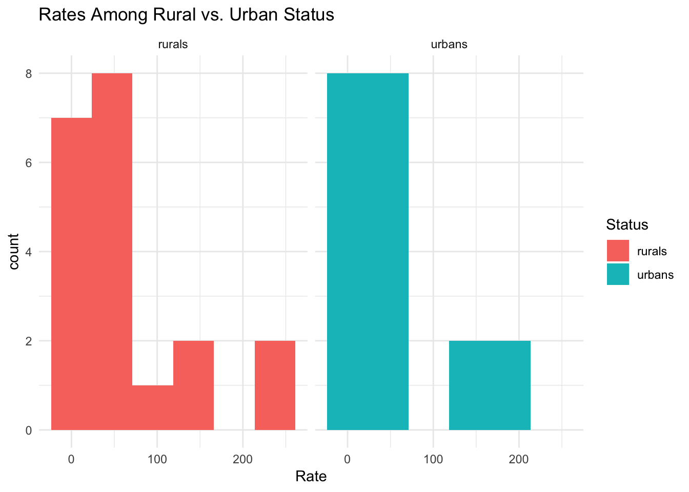
data1 %>%group_by(Status)%>%
summarize(means=mean(Rate))%>%summarize(`mean_diff:`=diff(means))
## # A tibble: 1 x 1
## `mean_diff:`
## <dbl>
## 1 -10.1Permutation Test
head(perm1<-data.frame(Status=data1$Status,Rate=sample(data1$Rate)))## Status Rate
## 1 rurals 21.8
## 2 rurals 34.9
## 3 rurals 71.3
## 4 rurals 24.7
## 5 rurals 17.7
## 6 rurals 49.6perm1%>%group_by(Status)%>%
summarize(means=mean(Rate))%>%summarize(`mean_diff:`=diff(means))## # A tibble: 1 x 1
## `mean_diff:`
## <dbl>
## 1 -5.38head(perm2<-data.frame(Status=data1$Status,Rate=sample(data1$Rate)))## Status Rate
## 1 rurals 44.5
## 2 rurals 36.1
## 3 rurals 12.9
## 4 rurals 210.2
## 5 rurals 19.4
## 6 rurals 6.2perm2%>%group_by(Status)%>%
summarize(means=mean(Rate))%>%summarize(`mean_diff:`=diff(means))## # A tibble: 1 x 1
## `mean_diff:`
## <dbl>
## 1 0.145rand_dist<-vector()
for(i in 1:5000){
new<-data.frame(Rate=sample(data1$Rate),Status=data1$Status)
rand_dist[i]<-mean(new[new$Status=="rurals",]$Rate)-
mean(new[new$Status=="urbans",]$Rate)}
{hist(rand_dist,main="",ylab=""); abline(v = -10.1,col="red")}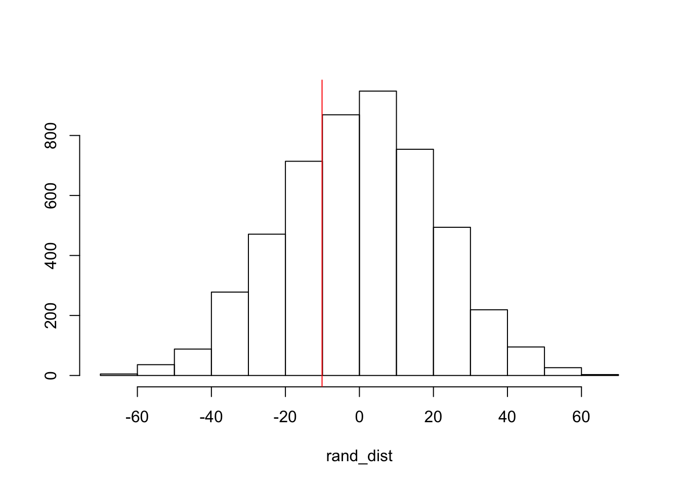
#p-value
mean(rand_dist>10.1)*2
## [1] 0.6328#t-test for comparison
t.test(data=data1,Rate~Status)##
## Welch Two Sample t-test
##
## data: Rate by Status
## t = 0.48183, df = 37.517, p-value = 0.6327
## alternative hypothesis: true difference in means is not equal to 0
## 95 percent confidence interval:
## -32.4009 52.6309
## sample estimates:
## mean in group rurals mean in group urbans
## 63.790 53.675H0 : mean rate of the deceased is the same for rural vs. urban status
HA : mean rate of the deceased differs among rural vs. urban status
This randomization test is scrambling the relationship between the variables rate and status. Due to this being a numeric by categorical, it was necessary to calculate the actual mean difference in the groups which was -10.1. The data was permuted twice in order to generated a sampling distrubution under our null hypothesis that it is false. It was then put into a for loop in order to generate this 5000 times as the randomization test. The p-value calculated means that there is a 0.6416 probability of observing a mean difference of as extreme as the one obtained from our randomization distribution. Based on our test statistic, there is not a significant difference that rate differs by status under this randomization test.
Logistic Regression
#mean centering 'Rate'
USMortality$Rate_c <- USMortality$Rate - mean(USMortality$Rate)

projectfit <- lm(Rate_c ~ Cause * Status, data = USMortality)
summary(projectfit)
##
## Call:
## lm(formula = Rate_c ~ Cause * Status, data = USMortality)
##
## Residuals:
## Min 1Q Median 3Q Max
## -43.9 -4.1 0.0 4.1 43.9
##
## Coefficients:
## Estimate Std. Error t value
## (Intercept) -32.53 17.52 -1.857
## CauseCancer 158.85 24.78 6.410
## CauseCerebrovascular diseases 16.00 24.78 0.646
## CauseDiabetes -0.55 24.78 -0.022
## CauseFlu and pneumonia -7.65 24.78 -0.309
## CauseHeart disease 172.60 24.78 6.965
## CauseLower respiratory 28.65 24.78 1.156
## CauseNephritis -10.10 24.78 -0.408
## CauseSuicide -9.95 24.78 -0.402
## CauseUnintentional injuries 28.05 24.78 1.132
## StatusUrban -3.75 24.78 -0.151
## CauseCancer:StatusUrban -13.25 35.04 -0.378
## CauseCerebrovascular diseases:StatusUrban -2.95 35.04 -0.084
## CauseDiabetes:StatusUrban -0.90 35.04 -0.026
## CauseFlu and pneumonia:StatusUrban 0.50 35.04 0.014
## CauseHeart disease:StatusUrban -23.70 35.04 -0.676
## CauseLower respiratory:StatusUrban -10.60 35.04 -0.302
## CauseNephritis:StatusUrban 0.85 35.04 0.024
## CauseSuicide:StatusUrban -0.25 35.04 -0.007
## CauseUnintentional injuries:StatusUrban -13.35 35.04 -0.381
## Pr(>|t|)
## (Intercept) 0.0782 .
## CauseCancer 2.97e-06 ***
## CauseCerebrovascular diseases 0.5258
## CauseDiabetes 0.9825
## CauseFlu and pneumonia 0.7607
## CauseHeart disease 9.24e-07 ***
## CauseLower respiratory 0.2612
## CauseNephritis 0.6879
## CauseSuicide 0.6923
## CauseUnintentional injuries 0.2710
## StatusUrban 0.8812
## CauseCancer:StatusUrban 0.7093
## CauseCerebrovascular diseases:StatusUrban 0.9338
## CauseDiabetes:StatusUrban 0.9798
## CauseFlu and pneumonia:StatusUrban 0.9888
## CauseHeart disease:StatusUrban 0.5066
## CauseLower respiratory:StatusUrban 0.7654
## CauseNephritis:StatusUrban 0.9809
## CauseSuicide:StatusUrban 0.9944
## CauseUnintentional injuries:StatusUrban 0.7073
## ---
## Signif. codes: 0 '***' 0.001 '**' 0.01 '*' 0.05 '.' 0.1 ' ' 1
##
## Residual standard error: 24.78 on 20 degrees of freedom
## Multiple R-squared: 0.9271, Adjusted R-squared: 0.8579
## F-statistic: 13.39 on 19 and 20 DF, p-value: 1.515e-07This linear regression model is prediciting the response variable ‘Rate_c’ from the variables, ‘Cause’ and ‘Status’. In this particular model, the original ‘Rate’ variable has been centered to result in a more informative interaction. The output of this model reveals that the intercept is an individual that was of a rural status and had a cause of death by Alzheimers. The intercept estimate reveals that people with a rural status and die by a cause of Alzheimers on average have an age-adjusted death rate of -32.53.
The coefficients of this model reveal the mean differences between the different groups and the intercept which is an individual that was a rural status and had a cause of death by Alzheimers. The coefficient ‘CauseCancer’ shows an average increase in the age-adjusted death rate by 158.85 and so does ‘CauseCerebrovascular diseases’ by 16.00. ‘CauseFlu and pneumonia’ shows an average decrease by ‘-7.65’ while ‘CauseDiabetes shows an average decrease by’-0.55’. The coefficient ‘CauseHeart disease’ reveals an average increase of 172.60 and ‘CauseLower respiratory’ shows an average increase of 28.65. An average decrease of -10.10 is shown by ‘CauseNephritis’ and ‘CauseSuicide’ reveals an average decrease of -9.95. The coefficient ‘CauseUnintentional injuries’ shows an average increase of 28.05. When an individual has the status of urban, they have an average age-adjusted death rate of -3.75.
It can be seen that the majority of the interactions have an average decrease, while only a few show an increase. A person that died due to a cause of cancer and had a status of urban had an average decrease of -13.25. A person that died due to cause of cerebrovascular diseases and had an urban status had an average decrease of -2.95. The coefficient ‘CauseDisease:StatusUrban’ shows an average disease of -0.90 while ‘CauseFlu and pneumonia:StatusUrban’ had an average increase of 0.50. ‘CauseHeart disease:StatusUrban’ showed that there was an average decrease of -23.50 while ‘CauseLower respiratory:StatusUrban’ also had an average decrease of -10.60. The coefficient ‘CauseNephritis:StatusUrban’ had an average increase of 0.85. When a person died by a cause of suicide and had an urban status, they showed an average decrease by -0.25 while those with an urban status and died by unintentional injuries had an average decrease by -13.35.
The two significant coefficients examinied in this models are cause by cancer and cause by heart disease. There is a significant effect of cause on rate dependendent on status.
#Formally testing heteroskedasticity assumptions
bptest(projectfit)
##
## studentized Breusch-Pagan test
##
## data: projectfit
## BP = 40, df = 19, p-value = 0.003272ggplot(USMortality, aes(Cause))+
geom_bar(aes(y=Rate_c,fill=Cause),
stat="summary", fun.y="mean")+
theme(axis.text.x = element_text(angle=45, hjust=1),
legend.position="none")+ ggtitle("Rate of Death By Different Causes")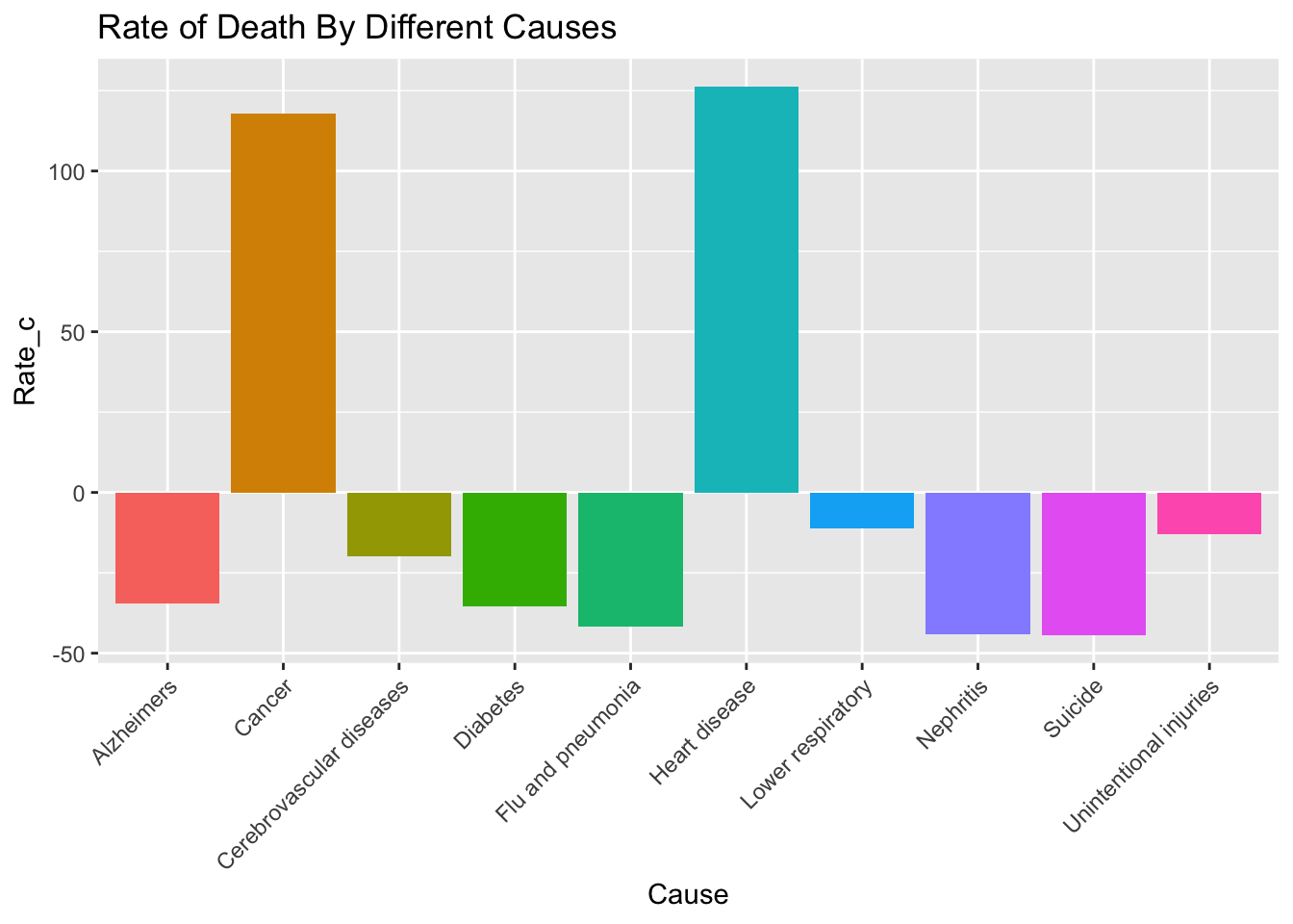
USMortality%>%ggplot(aes(Rate_c,Cause))+
geom_point()+geom_smooth(method = 'lm',se=F)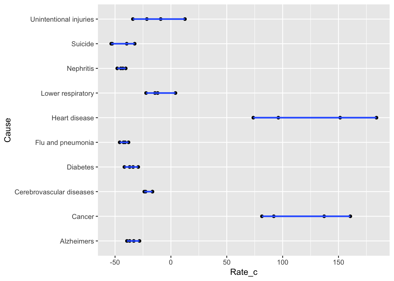
The best fitting line seen above is showing the predicted rate for an observation for a rural status that died by Alzheimers plus the estimate of each coefficient when it is “turned” on. For example, when an observation died by a cause of cancer then ‘CauseCancer’ is essentially “turned on” in our equation. Therefore, our intercept is increased by an average of 158.85.
ggplot(USMortality, aes(x=Rate_c, y=SE,group=Status))+geom_point(aes(color=Status))+
geom_smooth(method="lm",formula=y~1,se=F,fullrange=T,aes(color=Status))+theme(legend.position=c(.9,.19))+xlab("")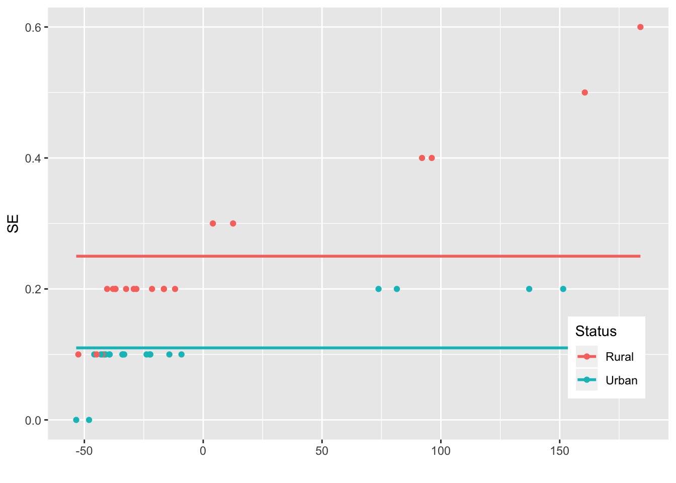
#Uncorrected SE's
summary(projectfit)$coef[,1:2]
## Estimate Std. Error
## (Intercept) -32.5325 17.52198
## CauseCancer 158.8500 24.77983
## CauseCerebrovascular diseases 16.0000 24.77983
## CauseDiabetes -0.5500 24.77983
## CauseFlu and pneumonia -7.6500 24.77983
## CauseHeart disease 172.6000 24.77983
## CauseLower respiratory 28.6500 24.77983
## CauseNephritis -10.1000 24.77983
## CauseSuicide -9.9500 24.77983
## CauseUnintentional injuries 28.0500 24.77983
## StatusUrban -3.7500 24.77983
## CauseCancer:StatusUrban -13.2500 35.04397
## CauseCerebrovascular diseases:StatusUrban -2.9500 35.04397
## CauseDiabetes:StatusUrban -0.9000 35.04397
## CauseFlu and pneumonia:StatusUrban 0.5000 35.04397
## CauseHeart disease:StatusUrban -23.7000 35.04397
## CauseLower respiratory:StatusUrban -10.6000 35.04397
## CauseNephritis:StatusUrban 0.8500 35.04397
## CauseSuicide:StatusUrban -0.2500 35.04397
## CauseUnintentional injuries:StatusUrban -13.3500 35.04397#Correct SE's (Robust Standard Errors)
coeftest(projectfit, vcov = vcovHC(projectfit))[,1:2]## Estimate Std. Error
## (Intercept) -32.5325 6.222540
## CauseCancer 158.8500 48.834875
## CauseCerebrovascular diseases 16.0000 6.222540
## CauseDiabetes -0.5500 8.268313
## CauseFlu and pneumonia -7.6500 6.988920
## CauseHeart disease 172.6000 62.395032
## CauseLower respiratory 28.6500 12.850097
## CauseNephritis -10.1000 6.957011
## CauseSuicide -9.9500 15.515315
## CauseUnintentional injuries 28.0500 24.902309
## StatusUrban -3.7500 7.571327
## CauseCancer:StatusUrban -13.2500 62.886366
## CauseCerebrovascular diseases:StatusUrban -2.9500 7.618727
## CauseDiabetes:StatusUrban -0.9000 10.834667
## CauseFlu and pneumonia:StatusUrban 0.5000 8.886507
## CauseHeart disease:StatusUrban -23.7000 83.248964
## CauseLower respiratory:StatusUrban -10.6000 14.687750
## CauseNephritis:StatusUrban 0.8500 8.916558
## CauseSuicide:StatusUrban -0.2500 18.866240
## CauseUnintentional injuries:StatusUrban -13.3500 30.801542#proportion of variation explained
summary(projectfit)$r.sq## [1] 0.9271126Based on the computation with robust standard errors, it can be seen that none of our estimates of the coefficients have changed but the standard errors have changed. The proportion of variance in the outcome that is explained by my model is 0.927.
BootStrapping
projectfit <- lm(Rate_c ~ Cause * Status, data = USMortality)
summary(projectfit)
##
## Call:
## lm(formula = Rate_c ~ Cause * Status, data = USMortality)
##
## Residuals:
## Min 1Q Median 3Q Max
## -43.9 -4.1 0.0 4.1 43.9
##
## Coefficients:
## Estimate Std. Error t value
## (Intercept) -32.53 17.52 -1.857
## CauseCancer 158.85 24.78 6.410
## CauseCerebrovascular diseases 16.00 24.78 0.646
## CauseDiabetes -0.55 24.78 -0.022
## CauseFlu and pneumonia -7.65 24.78 -0.309
## CauseHeart disease 172.60 24.78 6.965
## CauseLower respiratory 28.65 24.78 1.156
## CauseNephritis -10.10 24.78 -0.408
## CauseSuicide -9.95 24.78 -0.402
## CauseUnintentional injuries 28.05 24.78 1.132
## StatusUrban -3.75 24.78 -0.151
## CauseCancer:StatusUrban -13.25 35.04 -0.378
## CauseCerebrovascular diseases:StatusUrban -2.95 35.04 -0.084
## CauseDiabetes:StatusUrban -0.90 35.04 -0.026
## CauseFlu and pneumonia:StatusUrban 0.50 35.04 0.014
## CauseHeart disease:StatusUrban -23.70 35.04 -0.676
## CauseLower respiratory:StatusUrban -10.60 35.04 -0.302
## CauseNephritis:StatusUrban 0.85 35.04 0.024
## CauseSuicide:StatusUrban -0.25 35.04 -0.007
## CauseUnintentional injuries:StatusUrban -13.35 35.04 -0.381
## Pr(>|t|)
## (Intercept) 0.0782 .
## CauseCancer 2.97e-06 ***
## CauseCerebrovascular diseases 0.5258
## CauseDiabetes 0.9825
## CauseFlu and pneumonia 0.7607
## CauseHeart disease 9.24e-07 ***
## CauseLower respiratory 0.2612
## CauseNephritis 0.6879
## CauseSuicide 0.6923
## CauseUnintentional injuries 0.2710
## StatusUrban 0.8812
## CauseCancer:StatusUrban 0.7093
## CauseCerebrovascular diseases:StatusUrban 0.9338
## CauseDiabetes:StatusUrban 0.9798
## CauseFlu and pneumonia:StatusUrban 0.9888
## CauseHeart disease:StatusUrban 0.5066
## CauseLower respiratory:StatusUrban 0.7654
## CauseNephritis:StatusUrban 0.9809
## CauseSuicide:StatusUrban 0.9944
## CauseUnintentional injuries:StatusUrban 0.7073
## ---
## Signif. codes: 0 '***' 0.001 '**' 0.01 '*' 0.05 '.' 0.1 ' ' 1
##
## Residual standard error: 24.78 on 20 degrees of freedom
## Multiple R-squared: 0.9271, Adjusted R-squared: 0.8579
## F-statistic: 13.39 on 19 and 20 DF, p-value: 1.515e-07boot_dat<-USMortality[sample(nrow(USMortality),replace=TRUE),]
samp_distn<-replicate(5000, {
boot_dat<-USMortality[sample(nrow(USMortality),replace=TRUE),]
fit<- lm(Rate_c ~ Cause * Status, data = USMortality)
coef(fit)
})
#Bootstrapped SE's
samp_distn%>%t%>%as.data.frame%>%summarize_all(sd)## (Intercept) CauseCancer CauseCerebrovascular diseases CauseDiabetes
## 1 0 0 0 0
## CauseFlu and pneumonia CauseHeart disease CauseLower respiratory
## 1 0 0 0
## CauseNephritis CauseSuicide CauseUnintentional injuries StatusUrban
## 1 0 0 0 0
## CauseCancer:StatusUrban CauseCerebrovascular diseases:StatusUrban
## 1 0 0
## CauseDiabetes:StatusUrban CauseFlu and pneumonia:StatusUrban
## 1 0 0
## CauseHeart disease:StatusUrban CauseLower respiratory:StatusUrban
## 1 0 0
## CauseNephritis:StatusUrban CauseSuicide:StatusUrban
## 1 0 0
## CauseUnintentional injuries:StatusUrban
## 1 0samp_distn%>%t%>%as.data.frame%>%gather%>%group_by(key)%>%
summarize(lower=quantile(value,.025), upper=quantile(value,.975))## # A tibble: 20 x 3
## key lower upper
## <chr> <dbl> <dbl>
## 1 (Intercept) -32.5 -32.5
## 2 CauseCancer 159. 159.
## 3 CauseCancer:StatusUrban -13.3 -13.3
## 4 CauseCerebrovascular diseases 16. 16.
## 5 CauseCerebrovascular diseases:StatusUrban -2.95 -2.95
## 6 CauseDiabetes -0.55 -0.55
## 7 CauseDiabetes:StatusUrban -0.9 -0.9
## 8 CauseFlu and pneumonia -7.65 -7.65
## 9 CauseFlu and pneumonia:StatusUrban 0.500 0.500
## 10 CauseHeart disease 173. 173.
## 11 CauseHeart disease:StatusUrban -23.7 -23.7
## 12 CauseLower respiratory 28.6 28.6
## 13 CauseLower respiratory:StatusUrban -10.6 -10.6
## 14 CauseNephritis -10.1 -10.1
## 15 CauseNephritis:StatusUrban 0.850 0.850
## 16 CauseSuicide -9.95 -9.95
## 17 CauseSuicide:StatusUrban -0.25 -0.25
## 18 CauseUnintentional injuries 28.0 28.0
## 19 CauseUnintentional injuries:StatusUrban -13.4 -13.4
## 20 StatusUrban -3.75 -3.75Comparison
#Normal Standard Errors
coeftest(projectfit, vcov = vcovHC(projectfit))[,1:2]
## Estimate Std. Error
## (Intercept) -32.5325 6.222540
## CauseCancer 158.8500 48.834875
## CauseCerebrovascular diseases 16.0000 6.222540
## CauseDiabetes -0.5500 8.268313
## CauseFlu and pneumonia -7.6500 6.988920
## CauseHeart disease 172.6000 62.395032
## CauseLower respiratory 28.6500 12.850097
## CauseNephritis -10.1000 6.957011
## CauseSuicide -9.9500 15.515315
## CauseUnintentional injuries 28.0500 24.902309
## StatusUrban -3.7500 7.571327
## CauseCancer:StatusUrban -13.2500 62.886366
## CauseCerebrovascular diseases:StatusUrban -2.9500 7.618727
## CauseDiabetes:StatusUrban -0.9000 10.834667
## CauseFlu and pneumonia:StatusUrban 0.5000 8.886507
## CauseHeart disease:StatusUrban -23.7000 83.248964
## CauseLower respiratory:StatusUrban -10.6000 14.687750
## CauseNephritis:StatusUrban 0.8500 8.916558
## CauseSuicide:StatusUrban -0.2500 18.866240
## CauseUnintentional injuries:StatusUrban -13.3500 30.801542#Robust Standard Errors
coeftest(projectfit, vcov = vcovHC(projectfit))[,1:2]## Estimate Std. Error
## (Intercept) -32.5325 6.222540
## CauseCancer 158.8500 48.834875
## CauseCerebrovascular diseases 16.0000 6.222540
## CauseDiabetes -0.5500 8.268313
## CauseFlu and pneumonia -7.6500 6.988920
## CauseHeart disease 172.6000 62.395032
## CauseLower respiratory 28.6500 12.850097
## CauseNephritis -10.1000 6.957011
## CauseSuicide -9.9500 15.515315
## CauseUnintentional injuries 28.0500 24.902309
## StatusUrban -3.7500 7.571327
## CauseCancer:StatusUrban -13.2500 62.886366
## CauseCerebrovascular diseases:StatusUrban -2.9500 7.618727
## CauseDiabetes:StatusUrban -0.9000 10.834667
## CauseFlu and pneumonia:StatusUrban 0.5000 8.886507
## CauseHeart disease:StatusUrban -23.7000 83.248964
## CauseLower respiratory:StatusUrban -10.6000 14.687750
## CauseNephritis:StatusUrban 0.8500 8.916558
## CauseSuicide:StatusUrban -0.2500 18.866240
## CauseUnintentional injuries:StatusUrban -13.3500 30.801542#Bootstrapped Standard Errors
samp_distn%>%t%>%as.data.frame%>%summarize_all(sd)## (Intercept) CauseCancer CauseCerebrovascular diseases CauseDiabetes
## 1 0 0 0 0
## CauseFlu and pneumonia CauseHeart disease CauseLower respiratory
## 1 0 0 0
## CauseNephritis CauseSuicide CauseUnintentional injuries StatusUrban
## 1 0 0 0 0
## CauseCancer:StatusUrban CauseCerebrovascular diseases:StatusUrban
## 1 0 0
## CauseDiabetes:StatusUrban CauseFlu and pneumonia:StatusUrban
## 1 0 0
## CauseHeart disease:StatusUrban CauseLower respiratory:StatusUrban
## 1 0 0
## CauseNephritis:StatusUrban CauseSuicide:StatusUrban
## 1 0 0
## CauseUnintentional injuries:StatusUrban
## 1 0When comparing the normal standard errors, robust standard errors and the bootstrapped errors, we can see changes in the bootstrapped standard errors. There are no changes from the normal standard errors and the robust errors. THe only changes we see is in the bootstrapped standard errors and they are all 0’s.
Logistic Regression from Binary Variable
#Creating a Binary Variable
USMortality<- USMortality %>% mutate(y=ifelse(USMortality$Status=="Urban",1,0))


projectfit1 <- glm(y ~ Cause + Sex + Rate, data= USMortality,  family = "binomial")
summary(projectfit1)
##
## Call:
## glm(formula = y ~ Cause + Sex + Rate, family = "binomial", data = USMortality)
##
## Deviance Residuals:
## Min 1Q Median 3Q Max
## -1.62764 -1.07764 0.03858 1.05768 1.56117
##
## Coefficients:
## Estimate Std. Error z value Pr(>|z|)
## (Intercept) 0.76575 1.19965 0.638 0.5233
## CauseCancer 7.97061 4.44145 1.795 0.0727 .
## CauseCerebrovascular diseases 0.76447 1.53755 0.497 0.6190
## CauseDiabetes -0.05143 1.47005 -0.035 0.9721
## CauseFlu and pneumonia -0.38809 1.48799 -0.261 0.7942
## CauseHeart disease 8.39684 4.68743 1.791 0.0732 .
## CauseLower respiratory 1.23313 1.61404 0.764 0.4449
## CauseNephritis -0.50779 1.49765 -0.339 0.7346
## CauseSuicide -0.52844 1.48814 -0.355 0.7225
## CauseUnintentional injuries 1.11844 1.59361 0.702 0.4828
## SexMale 1.02491 0.81343 1.260 0.2077
## Rate -0.05260 0.02761 -1.905 0.0568 .
## ---
## Signif. codes: 0 '***' 0.001 '**' 0.01 '*' 0.05 '.' 0.1 ' ' 1
##
## (Dispersion parameter for binomial family taken to be 1)
##
## Null deviance: 55.452 on 39 degrees of freedom
## Residual deviance: 50.652 on 28 degrees of freedom
## AIC: 74.652
##
## Number of Fisher Scoring iterations: 4The above logistic regression model is predicting our binary variable urban status from the variables ‘Cause’, ‘Sex’ and ‘Rate’. In this model, the intercept is an observation that was female and died due to Alzheimers with a mean of 0.765 for urban status. The coefficient ‘CauseCancer’ reveals an 7.97 average increase when an observation died due to cancer. ‘CauseCerebrovascular diseases’ showed an average increase of 0.76 while ‘CauseDiabetes’showed an average decrease of -0.05. ’CauseFlu and pneumonia’ showed an average decrease of -0.38 while’CauseHeart disease’ showed an average increase of 8.38. ‘CauseLower respiratory’ showed an average increase of 1.23 while ‘CauseNephritis’ showed an average decrease of -0.50. ‘CauseSuicide’ showed an average decrease of -0.52 while the coefficient ‘CauseUnintentional injuries’ showed an average increase of 1.11. ‘SexMale’ showed an average incease of 1.02 and ‘Rate’ showed an average decrease of -0.05.
predict <- predict(projectfit1, type="response")
prob <- predict(projectfit1, type= "response")

USMortality<-USMortality%>%mutate(prob=predict(projectfit1, type="response"), prediction=ifelse(prob>.5,1,0))
classify<-USMortality%>%transmute(prob,prediction,truth=y)

#Confusion Matrix
table(predict=as.numeric(USMortality$prob>.5),truth=USMortality$y)%>%addmargins
## truth
## predict 0 1 Sum
## 0 13 8 21
## 1 7 12 19
## Sum 20 20 40#sensitivity
12/20## [1] 0.6#specificty
13/20## [1] 0.65#accuracy
(13+12)/40## [1] 0.625#precision
12/19## [1] 0.6315789According to the confusion matrix, the specificity calculated was 0.65 which is the proportion of urbans classified correctly. The sensitivity calculated was 0.6 which is the proportion of rurals properly classified. The overall accuracy of this confusion matrix ia 0.625 which specifies the proportion of correctly classified cases. The proportion of urbans who are actually urban and were classified as such was 0.631.
Density Plot
USMortality$logit <- predict(projectfit1, type="link")

USMortality%>%ggplot()+geom_density(aes(logit,color=y,fill=y), alpha=.4)+
theme(legend.position=c(.85,.85))+geom_vline(xintercept=0)+xlab("predictor (logit)")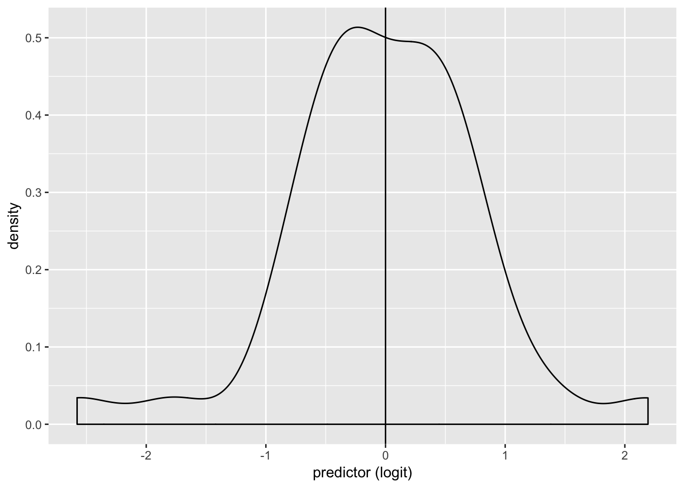
USMortality%>%ggplot()+geom_density(aes(logit,color=y,fill=Sex), alpha=.4)+
theme(legend.position=c(.85,.85))+geom_vline(xintercept=0)+xlab("predictor (logit)")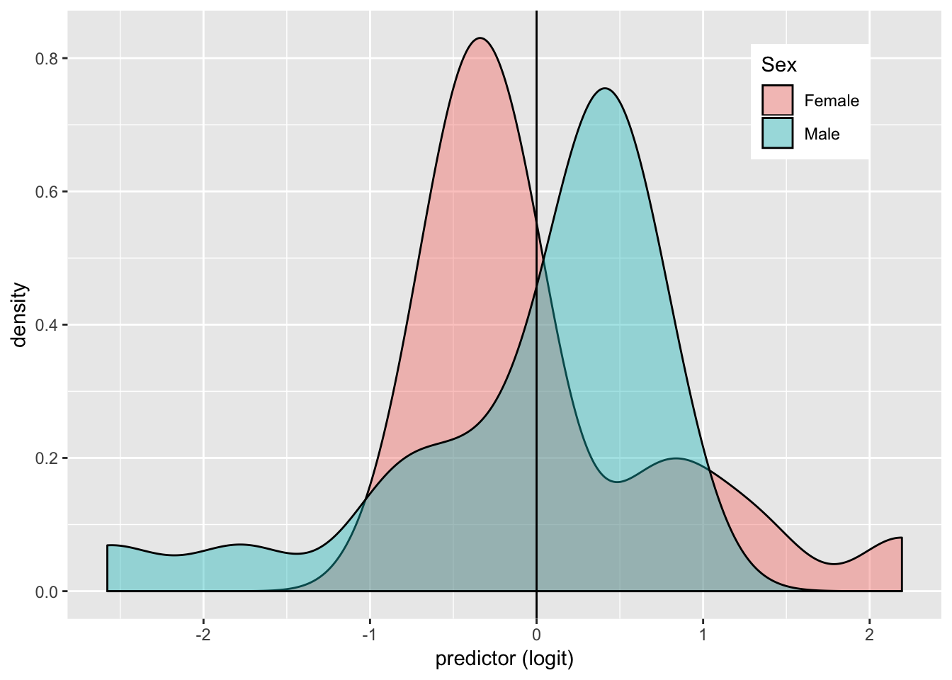
USMortality%>%ggplot()+geom_density(aes(logit,color=y,fill=Status), alpha=.4)+
theme(legend.position=c(.85,.85))+geom_vline(xintercept=0)+xlab("predictor (logit)")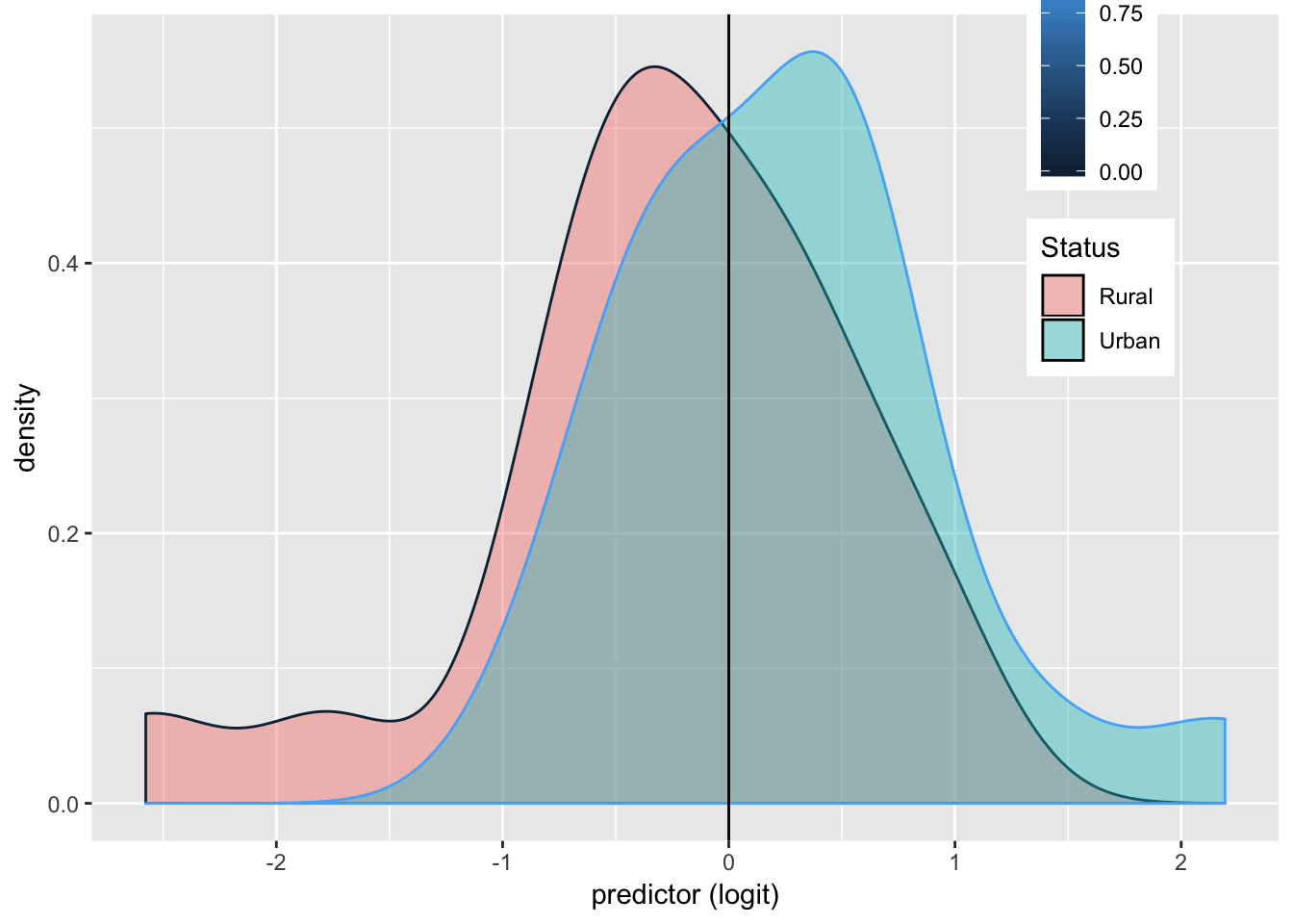
USMortality%>%ggplot()+geom_density(aes(logit,color=y,fill=Cause), alpha=.4)+
theme(legend.position=c(.85,.85))+geom_vline(xintercept=0)+xlab("predictor (logit)")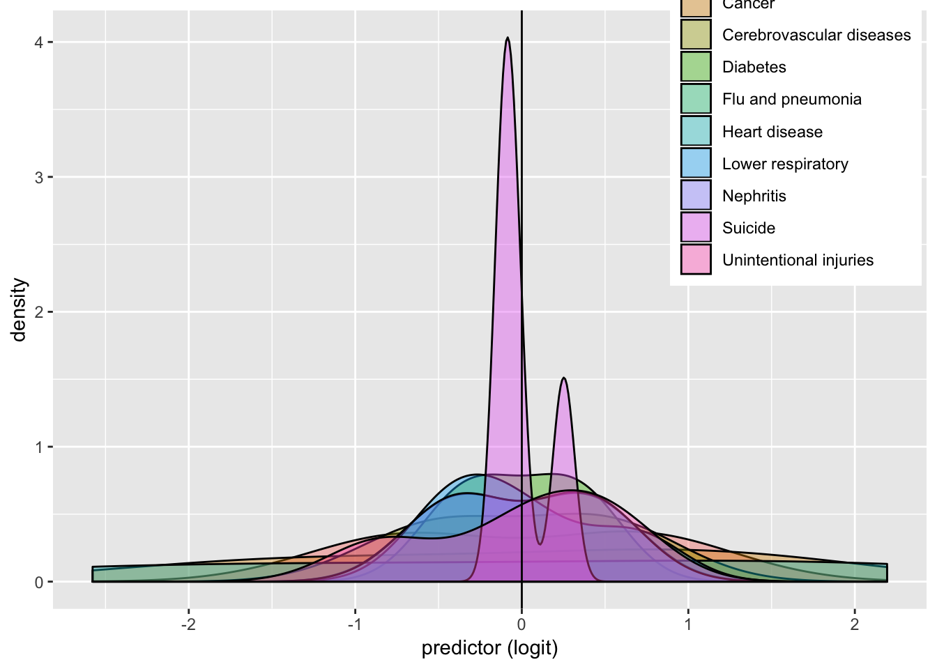
ROC Plot and AUC
ROCplot<-ggplot(USMortality)+geom_roc(aes(d=y,m=prob), n.cuts=0)
ROCplot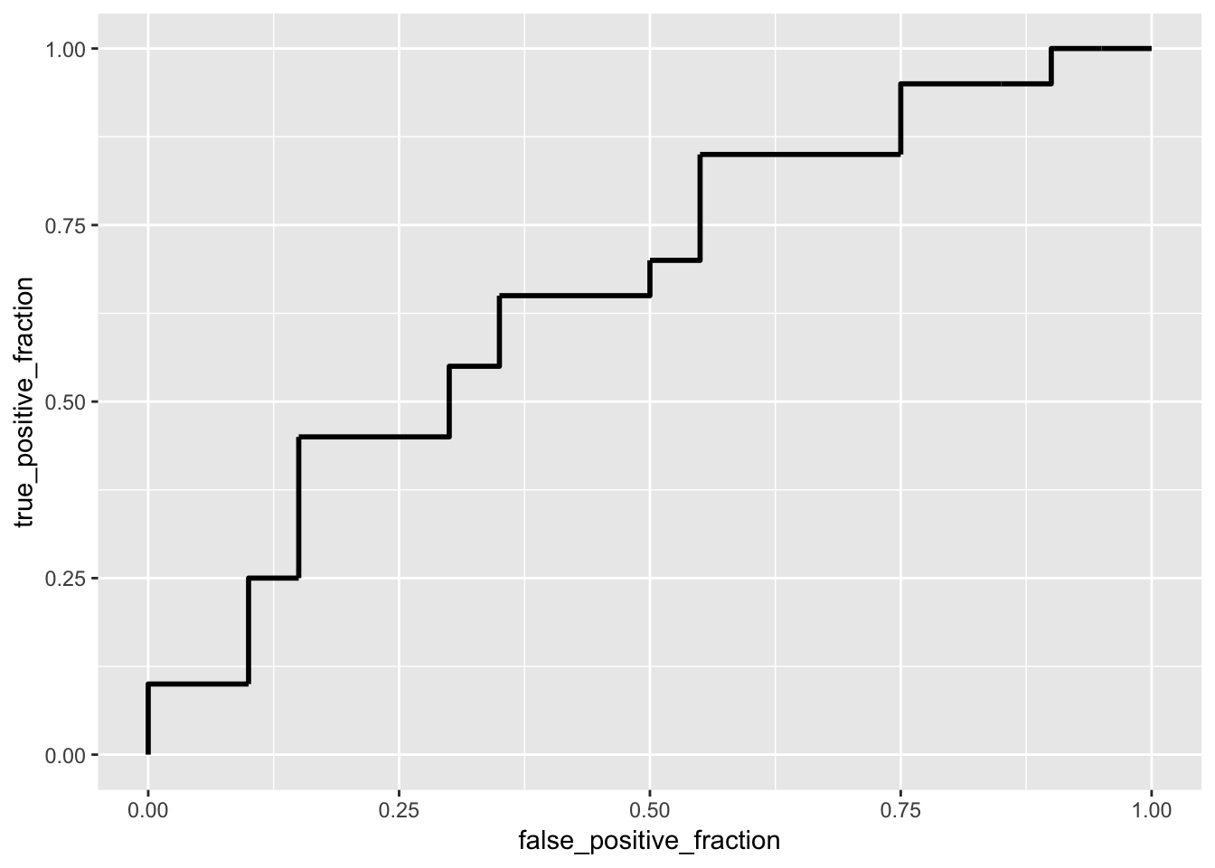
logs <- coef(projectfit1)%>%round(5)%>%data.frame

calc_auc(ROCplot)
## PANEL group AUC
## 1 1 -1 0.6625class_diag<-function(probs,truth){
tab<-table(factor(probs>.5,levels=c("FALSE","TRUE")),truth)
acc=sum(diag(tab))/sum(tab)
sens=tab[2,2]/colSums(tab)[2]
spec=tab[1,1]/colSums(tab)[1]
ppv=tab[2,2]/rowSums(tab)[2]
if(is.numeric(truth)==FALSE & is.logical(truth)==FALSE) truth<-as.numeric(truth)-1
ord<-order(probs, decreasing=TRUE)
probs <- probs[ord]; truth <- truth[ord]
TPR=cumsum(truth)/max(1,sum(truth))
FPR=cumsum(!truth)/max(1,sum(!truth))
dup<-c(probs[-1]>=probs[-length(probs)], FALSE)
TPR<-c(0,TPR[!dup],1); FPR<-c(0,FPR[!dup],1)
n <- length(TPR)
auc<- sum( ((TPR[-1]+TPR[-n])/2) * (FPR[-1]-FPR[-n]) )
data.frame(acc,sens,spec,ppv,auc)
}
#4-fold
set.seed(1234)
k=4
data1<-USMortality[sample(nrow(USMortality)),]
folds<-cut(seq(1:nrow(USMortality)),breaks=k,labels=F)
diags<-NULL
for(i in 1:k){
train<-data1[folds!=i,]
test<-data1[folds==i,]
truth<-test$y
fit<-glm(y ~ Cause + Sex + Rate, data= USMortality, family = "binomial")
probs<-predict(fit,newdata = test,type="response")
diags<-rbind(diags,class_diag(probs,truth))
}
apply(diags,2,mean)## acc sens spec ppv auc
## 0.6250000 0.6041667 0.6541667 0.6125000 0.7070833The generated ROC plot is split approximately down the middle which reveals that our model is not doing a good job at predicting overall. We are predicting only half well because if the ROC plot was closer to 1 then it would show that our model is predicting perfectly. The calculated AUC using the package has shown that the model is doing a poor job predicting overall as the value is 0.6625. After performing a 4-fold, the AUC increased to 0.707 which is now doing a fair job at predicting overall. A 4-fold was performed due to there being 40 observation which is relatively small, therefore it was necessary to set k equal to 4. After performing a 4-fold cross, this model is better at predicting status of an observation than the previous model.
LASSO Regression
projectfit2 <- glm(Sex~ -1 + (.), data = USMortality, family = "binomial")
model.matrix(projectfit2) %>% head()
## StatusRural StatusUrban CauseCancer CauseCerebrovascular diseases
## 1 0 1 0 0
## 2 1 0 0 0
## 3 0 1 0 0
## 4 1 0 0 0
## 5 0 1 1 0
## 6 1 0 1 0
## CauseDiabetes CauseFlu and pneumonia CauseHeart disease
## 1 0 0 1
## 2 0 0 1
## 3 0 0 1
## 4 0 0 1
## 5 0 0 0
## 6 0 0 0
## CauseLower respiratory CauseNephritis CauseSuicide
## 1 0 0 0
## 2 0 0 0
## 3 0 0 0
## 4 0 0 0
## 5 0 0 0
## 6 0 0 0
## CauseUnintentional injuries Rate SE Rate_c y prob prediction
## 1 0 210.2 0.2 151.4675 1 0.29563573 0
## 2 0 242.7 0.6 183.9675 0 0.07059824 0
## 3 0 132.5 0.2 73.7675 1 0.89967559 1
## 4 0 154.9 0.4 96.1675 0 0.73409044 1
## 5 0 195.9 0.2 137.1675 1 0.36765986 0
## 6 0 219.3 0.5 160.5675 0 0.14516786 0
## logit
## 1 -0.8681676
## 2 -2.5775358
## 3 2.1936252
## 4 1.0154760
## 5 -0.5422692
## 6 -1.7730144L <- model.matrix(projectfit2)
L <- scale(L)
M <- as.matrix(USMortality$Status)
cv3 <- cv.glmnet(L, M, family = "binomial")
lasso1 <- glmnet(L, M, family = "binomial", lambda = cv3$lambda.1se)
coef(lasso1)## 19 x 1 sparse Matrix of class "dgCMatrix"
## s0
## (Intercept) -2.382550e-15
## StatusRural -7.390803e+00
## StatusUrban 2.577618e-15
## CauseCancer .
## CauseCerebrovascular diseases .
## CauseDiabetes .
## CauseFlu and pneumonia .
## CauseHeart disease .
## CauseLower respiratory .
## CauseNephritis .
## CauseSuicide .
## CauseUnintentional injuries .
## Rate .
## SE .
## Rate_c .
## y 4.833033e-16
## prob .
## prediction .
## logit .#4-Fold
set.seed(1234)
k=4
data2<-USMortality[sample(nrow(USMortality)),]
folds<-cut(seq(1:nrow(USMortality)),breaks=k,labels=F)
diags<-NULL
for(i in 1:k){
train<-data2[folds!=i,]
test<-data2[folds==i,]
truth<-test$Sex
fit2<-glm(Sex~ Status ,data=USMortality,family="binomial")
probs<-predict(fit2,newdata = test,type="response")
diags<-rbind(diags,class_diag(probs,truth))
}
diags%>%summarize_all(mean)## acc sens spec ppv auc
## 1 0.5 0.5208333 0.4916667 0.5083333 0.50625After performing a LASSO regression, it can be seen that the variables that are retained and are significant in predicting the sex of an observation is ‘StatusRural’ , ‘StatusUrban’ and the binary variable y. It can be seen that this model is not doing a good job at predicting and fitting overall values. Therefore, this model should not be used to fit new data because it is doing a bad job at prediting overall due to the AUC being 0.505.