January 1, 0001
Project 1: Exploratory Data Analysis
Desiree Lama: dl33464
Introduction
The two datasets that have been used in the following data analysis involve music analyzation. The first data set is titled ‘kpopreal’ which was acquired from my prior BioStatistics project where I was testing to determine if there was a correlation between race and Kpop. The variables in the ‘kpopreal’ dataset are Groups.Artists, Genre, Race and Subject. The ‘Groups.Artists’ variable was viewing the number of Kpop groups/artists that the subject knew from a generated list of Kpop artists. The ‘Race’ variable includes the associated race of the subject and the ‘Genre’ variable asked the subject which genre of music are they most likely to listen to outside of Kpop from rap, country, indie, rock and hip-hop. The ‘Subject’ variable numbers the participants from 1-139. The second dataset that is used in this data analysis is called ‘MusicTime’. This dataset contains 60 observations with 6 different variables. This particular study requested the participants to judge when 45 seconds of silence had passed which was the control. They were also asked to determine when 45 seconds of an upbeat and calm song had passed. The variables in the ‘MusicTime’ dataset are MusicBg, Subject, Sex, TimeGuess, Music and Accuracy. The variable ‘MusicBg’ determines whether music playing or not, ‘Subject’ numbers the participants from 1-60 and ‘Sex’ recorded if the participant is male or female. The ‘TimeGuess’ variable measures the subject’s time in estimating 45 seconds and ‘Music’ marked if the music was playing was either calm, control or upbeat music. The last variable, ‘Accuracy’ is the absolute value of variable ‘TimeGuess’ minus 45. These two datasets were interesting to me because they are both associated with music. Music is a universal language for all and has the capability of uniting people of various cultures and ethnicites, therefore choosing to analyze datasets that are examining music was a key decision factor for me. Associations that are expected to be found upon analyzing these datasets further is there will be a difference in the amount of Kpop groups that a subject knows based on race and the accuracy of their time guess depends on the music being played.
Packages Used in Data Analysis
library(plyr)
library(dplyr)
library(tidyr)
library(tidyverse)
library(factoextra)
library(readr)
Importing ‘kpopreal’ Dataset
library(readr)
kpopreal <- read.csv("~/Downloads/kpopreal.csv")
Untidying ‘kpopreal’ Dataset
kpopreal1 <- kpopreal %>% pivot_wider(names_from = "Race1", values_from = "NumberOfArtists")

kpopreal1 <- kpopreal1 %>% pivot_wider(names_from = "Groups.Artists", values_from ="Genre1")
Due to the ‘kpopreal’ dataset being tidy, it was necessary to untidy them by using tidyr adn tidyverse functions. The main function that was used in order to untidy the ‘kpopreal’ dataset was the pivot_wider function. The ‘kpopreal’ dataset was saved into ‘kpopreal1’ then piped into pivot_wider which took the races that were under the ‘Race1’ column and migrated them into their own individual columns. Continuing this untidying process, another piping was done using pivot_wider by piping ‘kpopreal1’ into pivot_wider and shifting the groups that were originally located under the ‘Groups.Artists’ column into their own variable columns.The resulting dataset is an untidy dataframe that now contains 48 variables which include ‘Subject’, ‘American Indian’, ‘Asian’, ‘Black or African American’, ‘Native Hawaiian or Other Pacific Islander’, ‘White’ and the various of different combinations of answers that the subject’s responded to the survey of their knowledge of Kpop groups and artists.
Tidying ‘kpopreal’ Data
kpoprealtidy <- kpopreal1 %>% pivot_longer(2:6,names_to = "Race")

kpoprealtidy <- kpoprealtidy %>%
pivot_longer(cols=-c("Subject","Race","value"), names_repair = "check_unique", names_to = "Groups/Artists", values_to = "Genre")

kpoprealtidy <- kpoprealtidy %>% na.omit()
kpoprealtidy <- kpoprealtidy %>% rename("NumberOfArtists" = value)
Following untidying the ‘kpopreal’ dataset, the dataframe required tidying using tidyr and tidyverse functions as well. The first step in the tidying process involved using the function pivot_longer by piping ‘kpopreal1’ into pivot_longer, selecting the columns 2 through 6 only in order to rename them into a ‘Race’ column and saving this into ‘kpoprealtidy’. The following step also included piping ‘kpoprealtidy’ into pivot_longer. The columns ‘Subject’, ‘Race’, and “value’ were disselected while the remaining columns were inserted into a columns named ‘Groups/Artists’ and ‘Genre’. The function names_repair was necessary in order to ensure that there were no duplicate columns. The dataset then required the ommitance of NA’s through the usage of na.omit(). Subsequently, ‘kpoprealtidy’ was resaved renaming the column ‘value’ into ‘NumberOfArtists’.
Importing ‘MusicTime’ Dataset
MusicTime <- read.csv("~/Downloads/MusicTime.csv")

MusicTime <- MusicTime %>% select(-X, -Subject)
MusicTime <- MusicTime %>% add_column(Subject=1:60)
It was necessary to disselect the columns ‘X’ and ‘Subject’ from the ‘MusicTime’ dataset and override it into ‘MusicTime’. It was also required to created a column for ‘Subject’ that numbered the subjects from 1-60 for a later join.
Untidying the ‘MusicTime’
MT <- MusicTime %>% pivot_wider(names_from = "Sex", values_from = "TimeGuess")
MT1 <- MT %>% pivot_wider(names_from = "MusicBg", values_from = "Subject")
The ‘MusicTime’ dataset required untidying through tidyr and tidyverse functions. The first step in this process was piping ‘MusicTime’ into pivot_wider which separated the sex of the subjects into distinct columns with their corresponding ‘TimeGuess’. Thereafter saving this command into ‘MT’, another pivot_wider code was necessary to further divide the variable into distinct columns. The following command that was ran was piping ‘MT’ into pivot_wider which then created a ‘yes’ and ‘no’ column originating from ‘MusicBg’.
Tidying the ‘MusicTime’ Data
MT1 <- MT1 %>% pivot_longer(3:4, names_to = "Sex")
MT1 <- MT1 %>% pivot_longer(3:4, names_repair = "check_unique" , names_to = "MusicBg" , values_to = "Subject")
MT1 <- MT1 %>% na.omit()
In order to tidy the ‘MT1’ dataset, tidyr functions were essential. Initially, it is necessary to pipe ‘MT1’ into the function pivot_longer selecting the columns 3 through 4 and renaming them into ‘Sex’ and overriding that into ‘MT1’. The next step is to pipe ‘MT1’ into pivot_longer selecting columns 3 through 4 which will create the columns ‘MusicBg’ and ‘Subject’. The names_repair function is necessary in order to ensure that there are no duplicate in columns when forming the two new columns ‘MusicBg’ and ‘Subject’. The final task is to override MT1 and pipe it into na.omit #in order to remove the NA’s from the dataset.
Joining ‘kpopreal’ and ‘MusicTime’ Datasets using a right join
fulldata <- right_join(kpopreal, MusicTime)To join the ‘kpopreal’ and ‘MusicTime’ datasets into one combined dataset, the the dplyr right_join function was required. The reason behind using a right_join was because there were cases in each dataset that did not have a match which would result in dropping of NA’s. The two datasets were joined by the variable ‘Subject’ and the resulting joined dataset was saved into ‘fulldata’. The cases that were dropped were all the subjects that identified as White, Native Hawaiian or Other Pacific Islander and 6 of the Black or African American subjects. An arising issue that could potentially be faced with this is the subjects that are White will not be represented in the data, therefore the data could inaccurately exhibit correlations between the variables.
Summary Statistics
1## [1] 1fulldata %>% group_by(Genre1, Race1)%>% summarize(mean_NumberOfArtists=mean(NumberOfArtists, na.rm=T),
n_rows=n(), n_TimeGuess=n_distinct(Race1))## # A tibble: 10 x 5
## # Groups: Genre1 [5]
## Genre1 Race1 mean_NumberOfArtis… n_rows n_TimeGuess
## <fct> <fct> <dbl> <int> <int>
## 1 Country Asian 6.5 2 1
## 2 Hip Hop American Indian 2 1 1
## 3 Hip Hop Asian 6.27 15 1
## 4 Hip Hop Black or African American 8 4 1
## 5 Indie American Indian 6.5 2 1
## 6 Indie Asian 5.77 13 1
## 7 Rap American Indian 7 4 1
## 8 Rap Asian 6.2 5 1
## 9 Rock American Indian 4 2 1
## 10 Rock Asian 6.67 12 12## [1] 2fulldata %>% summarize(mean_NumberOfArtists=mean(NumberOfArtists, na.rm=T),
n_rows=n(), n_Race1=n_distinct(Race1))## mean_NumberOfArtists n_rows n_Race1
## 1 6.266667 60 33## [1] 3fulldata %>% group_by(Race1)%>% summarize(mean_NumberOfArtists=mean(NumberOfArtists, na.rm=T),
n_rows=n(), n_TimeGuess=n_distinct(Race1))## # A tibble: 3 x 4
## Race1 mean_NumberOfArtists n_rows n_TimeGuess
## <fct> <dbl> <int> <int>
## 1 American Indian 5.67 9 1
## 2 Asian 6.23 47 1
## 3 Black or African American 8 4 14## [1] 4fulldata %>% summarize_all(n_distinct)## Groups.Artists Genre1 Race1 NumberOfArtists Subject MusicBg Sex
## 1 26 5 3 9 60 2 2
## TimeGuess Music Accuracy
## 1 42 3 315## [1] 5fulldata %>% mutate(`Accuracy_pctile`=ntile(Accuracy,100)) %>% glimpse()## Observations: 60
## Variables: 11
## $ Groups.Artists <fct> BTS;Red Velvet, BTS;Dean;SHINee;Red Velvet, NU'E…
## $ Genre1 <fct> Hip Hop, Indie, Indie, Rap, Rap, Rap, Rap, Rock,…
## $ Race1 <fct> American Indian, American Indian, American India…
## $ NumberOfArtists <int> 2, 4, 9, 7, 7, 7, 7, 1, 7, 8, 5, 8, 4, 1, 6, 8, …
## $ Subject <int> 1, 2, 3, 4, 5, 6, 7, 8, 9, 10, 11, 12, 13, 14, 1…
## $ MusicBg <fct> yes, no, no, yes, yes, yes, yes, yes, no, no, ye…
## $ Sex <fct> m, f, f, f, m, m, f, m, m, m, f, m, f, m, m, m, …
## $ TimeGuess <int> 43, 18, 68, 26, 40, 47, 29, 38, 29, 41, 36, 23, …
## $ Music <fct> control, control, control, control, control, con…
## $ Accuracy <int> 2, 27, 23, 19, 5, 2, 16, 7, 16, 4, 9, 22, 7, 3, …
## $ Accuracy_pctile <int> 2, 87, 81, 69, 22, 4, 56, 31, 57, 16, 39, 74, 32…6## [1] 6fulldata %>% mutate(`TimeGuess_pctile`=ntile(TimeGuess,100)) %>% glimpse()## Observations: 60
## Variables: 11
## $ Groups.Artists <fct> BTS;Red Velvet, BTS;Dean;SHINee;Red Velvet, NU'…
## $ Genre1 <fct> Hip Hop, Indie, Indie, Rap, Rap, Rap, Rap, Rock…
## $ Race1 <fct> American Indian, American Indian, American Indi…
## $ NumberOfArtists <int> 2, 4, 9, 7, 7, 7, 7, 1, 7, 8, 5, 8, 4, 1, 6, 8,…
## $ Subject <int> 1, 2, 3, 4, 5, 6, 7, 8, 9, 10, 11, 12, 13, 14, …
## $ MusicBg <fct> yes, no, no, yes, yes, yes, yes, yes, no, no, y…
## $ Sex <fct> m, f, f, f, m, m, f, m, m, m, f, m, f, m, m, m,…
## $ TimeGuess <int> 43, 18, 68, 26, 40, 47, 29, 38, 29, 41, 36, 23,…
## $ Music <fct> control, control, control, control, control, co…
## $ Accuracy <int> 2, 27, 23, 19, 5, 2, 16, 7, 16, 4, 9, 22, 7, 3,…
## $ TimeGuess_pctile <int> 32, 1, 84, 6, 26, 39, 12, 24, 14, 31, 22, 4, 56…7## [1] 7fulldata %>% summarize(mean_TimeGuess=mean(TimeGuess, na.rm=T),
n_rows=n(),
n_race=n_distinct(Race1))## mean_TimeGuess n_rows n_race
## 1 51 60 38## [1] 8fulldata %>% filter(Genre1 == "Hip Hop",Sex=="f") %>%
arrange(desc(NumberOfArtists)) %>% glimpse()## Observations: 12
## Variables: 10
## $ Groups.Artists <fct> NU'EST;Ailee;BTS;Twice;The Rose;Dean;SHINee;Red …
## $ Genre1 <fct> Hip Hop, Hip Hop, Hip Hop, Hip Hop, Hip Hop, Hip…
## $ Race1 <fct> Asian, Black or African American, Asian, Asian, …
## $ NumberOfArtists <int> 9, 9, 8, 8, 8, 8, 8, 8, 7, 5, 4, 2
## $ Subject <int> 23, 57, 18, 19, 20, 22, 58, 60, 59, 17, 13, 24
## $ MusicBg <fct> no, yes, yes, no, yes, no, yes, yes, no, yes, no…
## $ Sex <fct> f, f, f, f, f, f, f, f, f, f, f, f
## $ TimeGuess <int> 67, 33, 21, 33, 48, 28, 94, 49, 51, 27, 52, 49
## $ Music <fct> upbeat, calm, control, control, control, upbeat,…
## $ Accuracy <int> 22, 12, 24, 12, 3, 17, 49, 4, 6, 18, 7, 49## [1] 9fulldata %>% mutate(Accuracy_quartile=ntile(Accuracy,4)) %>% head()## Groups.Artists Genre1
## 1 BTS;Red Velvet Hip Hop
## 2 BTS;Dean;SHINee;Red Velvet Indie
## 3 NU'EST;Ailee;BTS;Twice;The Rose;Dean;SHINee;Red Velvet;Got7 Indie
## 4 NU'EST;BTS;Twice;Dean;SHINee;Red Velvet;Got7 Rap
## 5 Ailee;BTS;Twice;Dean;SHINee;Red Velvet;Got7 Rap
## 6 NU'EST;Ailee;BTS;Twice;SHINee;Red Velvet;Got7 Rap
## Race1 NumberOfArtists Subject MusicBg Sex TimeGuess Music
## 1 American Indian 2 1 yes m 43 control
## 2 American Indian 4 2 no f 18 control
## 3 American Indian 9 3 no f 68 control
## 4 American Indian 7 4 yes f 26 control
## 5 American Indian 7 5 yes m 40 control
## 6 American Indian 7 6 yes m 47 control
## Accuracy Accuracy_quartile
## 1 2 1
## 2 27 4
## 3 23 4
## 4 19 3
## 5 5 1
## 6 2 110## [1] 10z_score<-function(x)(x-mean(x, na.rm=T))/sd(x, na.rm=T)
fulldata %>% mutate_at(c("TimeGuess","Accuracy"),z_score) %>% arrange(desc(TimeGuess,Accuracy)) %>% glimpse()## Observations: 60
## Variables: 10
## $ Groups.Artists <fct> BTS;SHINee, NU'EST;Ailee;BTS;Twice;Dean;SHINee;R…
## $ Genre1 <fct> Rock, Hip Hop, Rap, Indie, Rock, Rock, Rock, Roc…
## $ Race1 <fct> Asian, Black or African American, Asian, Asian, …
## $ NumberOfArtists <int> 2, 8, 8, 6, 4, 9, 8, 7, 9, 6, 9, 9, 8, 5, 9, 1, …
## $ Subject <int> 53, 58, 43, 33, 45, 49, 54, 46, 3, 29, 23, 47, 5…
## $ MusicBg <fct> no, yes, no, no, yes, no, no, yes, no, no, no, y…
## $ Sex <fct> f, f, f, f, m, m, m, m, f, m, f, f, m, m, f, m, …
## $ TimeGuess <dbl> 2.68388602, 2.35524692, 2.30047373, 1.64319552, …
## $ Music <fct> calm, calm, calm, upbeat, calm, calm, calm, calm…
## $ Accuracy <dbl> 3.33095867, 2.83297482, 2.74997751, 1.75400980, …11## [1] 11fulldata %>% select(-Groups.Artists, -Genre1, -Race1, -MusicBg, -Music, -Sex) %>% summarize_all(n_distinct)## NumberOfArtists Subject TimeGuess Accuracy
## 1 9 60 42 3112## [1] 12fulldata %>% summarize(cor(TimeGuess,Accuracy))## cor(TimeGuess, Accuracy)
## 1 0.590983513## [1] 13dframe <- fulldata %>% select(-Subject) %>% select_if(is.numeric)
cor(dframe)## NumberOfArtists TimeGuess Accuracy
## NumberOfArtists 1.00000000 0.08532303 0.08865022
## TimeGuess 0.08532303 1.00000000 0.59098350
## Accuracy 0.08865022 0.59098350 1.00000000corrl <- cor(dframe) %>% as.data.frame %>%
rownames_to_column %>% pivot_longer(-1,names_to="name",values_to="correlation")Correlation Matrix Visualized
corrl%>%ggplot(aes(rowname,name,fill=correlation))+
     geom_tile()+
     scale_fill_gradient2(low="pink",mid="white",high="purple")+
     geom_text(aes(label=round(correlation,2)),color = "black", size = 4)+
     theme(axis.text.x = element_text(angle = 90, hjust = 1))+
coord_fixed() 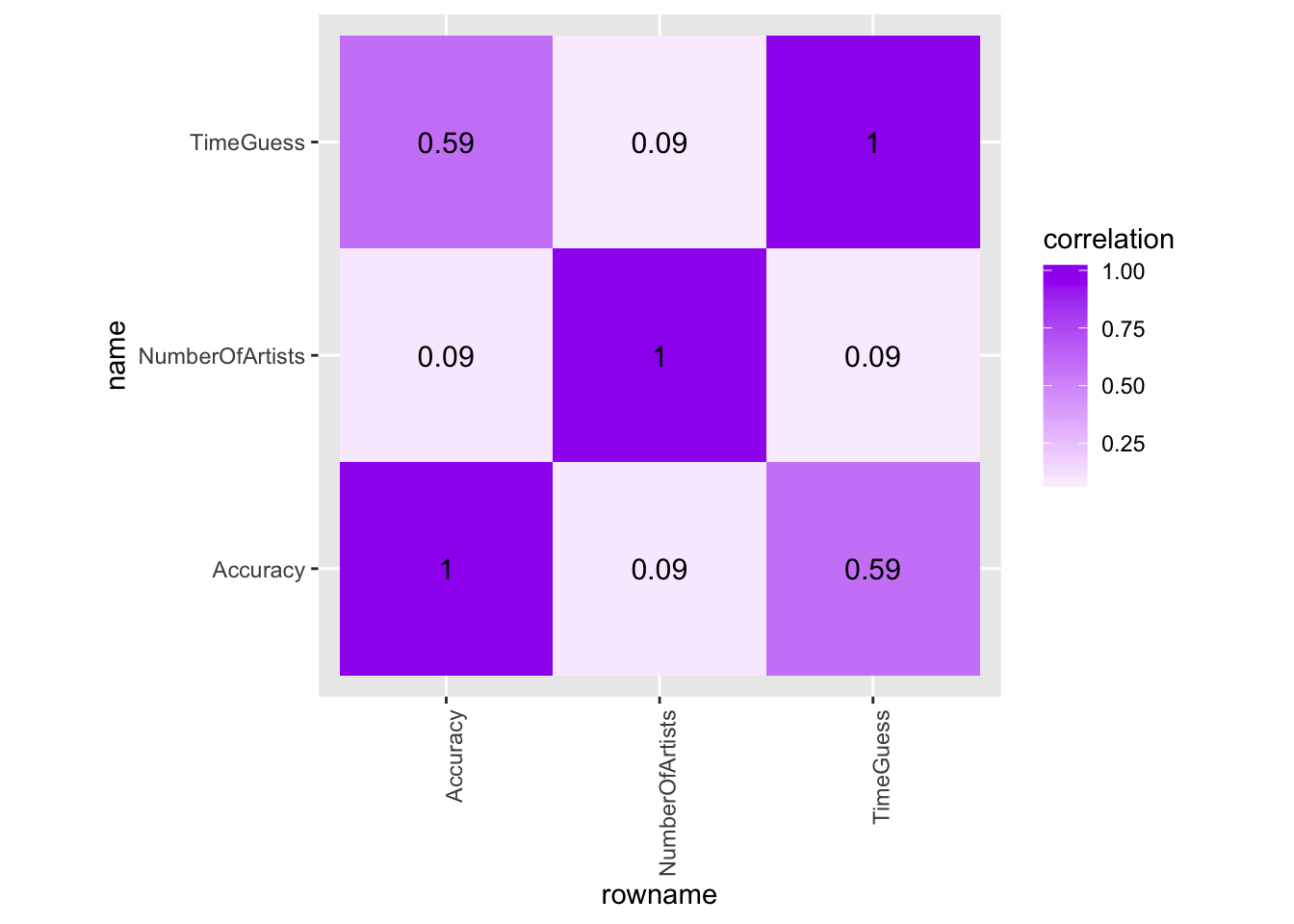
Through the use of dplyr functions, the joined ‘kpopreal’ and ‘MusicTime’ dataset have been explored in order to compute a variety of summary statistics. Through these summary statistics, it can be seen that the average time guess for a 45 second interval was 51 seconds. The mean number of groups and artists that a subject knew was approximately 6 which varied among the races. The Black/African Americans subjects on avergae knew the most groups and artists with a mean of 8 and American Indians knew the least with a mean of 5.67. Through the correlation matrix it can be seen that the highest correlation is between the variables ‘TimeGuess’ and ‘Accuracy’. The lowest correlation that is depicted is ‘NumberOfArtists’ with ‘Accuracy’ and ‘TimeGuess’. Overall, it is seen that the correlations are highest between the variables that are observed in the study.
Visualizations
ggplot(fulldata, aes(x = Race1, y = TimeGuess))+
  geom_bar(aes(fill=Race1), stat="summary",fun.y="mean")+
  geom_errorbar(stat="summary") + scale_x_discrete("Race", breaks = seq(0,60, by = 5)) +
  ggtitle("Time Guess by Race") + scale_fill_brewer(palette = "Reds") + facet_wrap(~Sex)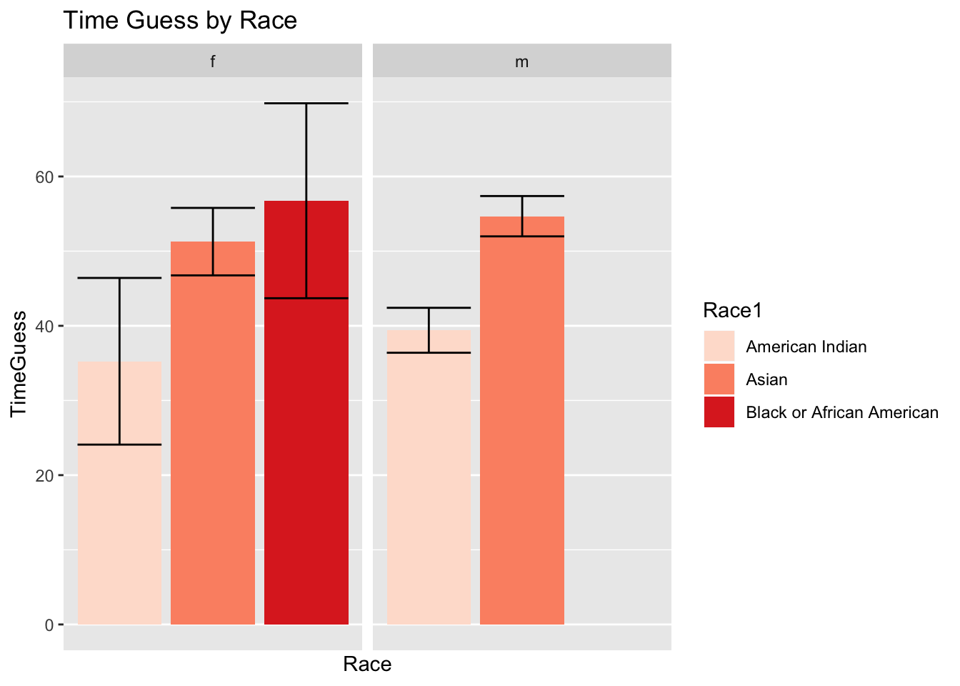
The bar graph above illustrates time guesses categorized by the three different races: American Indian, Asian and Black or African American faceted by male and female. It can be seen that the female subjects who identify as Black/African American and Asian have relatively close time guesses compared to American Indian females. The bar graph also depicts that Asian males differ from American Indian males, while there were no Black/African American male subjects. The standard errors bars that are shown for female American Indian and Black/African Americans are fairly large which indicates variability in the data. The remaining standard error bars for female Asian subjects and male American Indians and Black/African Americans are rather smaller in comparison to the others, which shows that there is less uncertainty reported for these specific groups. When comparing males and females to each other, there is no major difference in the average time guesses among the different races.
ggplot(data=fulldata) + geom_point(mapping = aes(x=TimeGuess, y=Accuracy,
  shape= Sex, color = NumberOfArtists)) +
  ggtitle("Accuracy of Time Guesses Based on Sex") + theme_linedraw() +
  scale_color_gradient2(low="blue",mid="white",high="purple") + facet_wrap(~Genre1)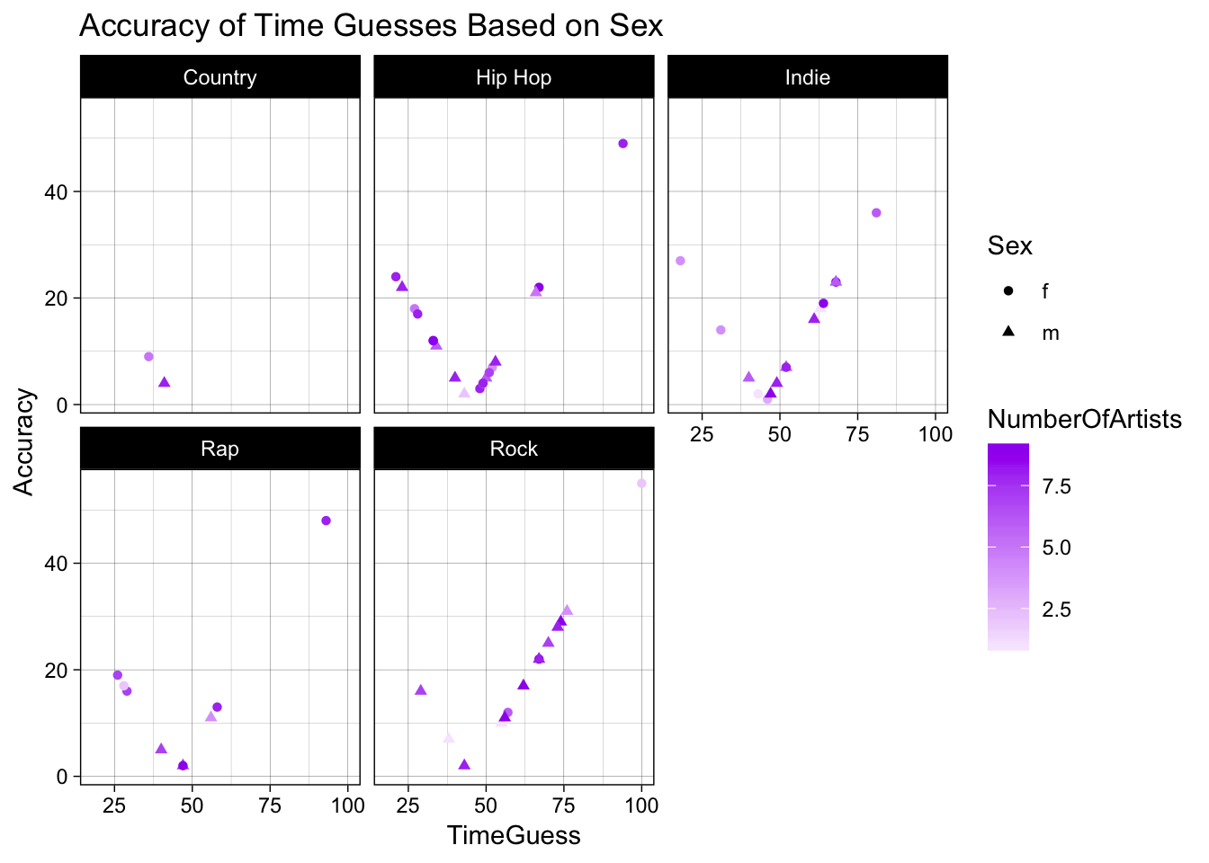
The plots above depicts the accuracy of time guesses of music played in the study based on the sex of a subject separated by the type of music they are most likely to listen to outside of Kpop. The plots also represents the number of artists of Kpop artists and groups that the subject knew through the color of the point. From first glance, it can be seen that there were a large majority of participants that listen to hip-hop, indie and rock music outside of Kpop while fewer listen to country. A majority of both male and female subjects knew around 5 and 7 kpop groups and artists according to the colors that are indicated by the points. It is also revealed that the number of artists across both male and female appears to be relatively constant. There is a general trend that the longer a subject takes in guessing a 45 second interval, the higher their aaccuracy will be. The shorter the amount of time a participant took to guess a 45 second time interval the less accurate they tended to be. The subjects among each genre of music portrayed various of knowledge in the amount of Kpop artists and groups that they knew.
Principal Component Analysis
fulldata%>%select_if(is.numeric)%>%scale%>%prcomp->f_pca

summary(f_pca, loadings = T)
## Importance of components:
## PC1 PC2 PC3 PC4
## Standard deviation 1.4107 0.9918 0.8421 0.56300
## Proportion of Variance 0.4975 0.2459 0.1773 0.07924
## Cumulative Proportion 0.4975 0.7435 0.9208 1.00000eigenvals <- f_pca$sdev^2
varprop=round(eigenvals/sum(eigenvals),2)
ggplot()+geom_bar(aes(x=1:4,y=varprop),stat="identity")+xlab("")+geom_path(aes(y=varprop,x=1:4))+geom_text(aes(x=1:4,y=varprop,label=round(varprop,2)),vjust=1,col="white",size=5)+scale_y_continuous(breaks=seq(0,.6,.2),labels = scales::percent)+ scale_x_continuous(breaks=1:10)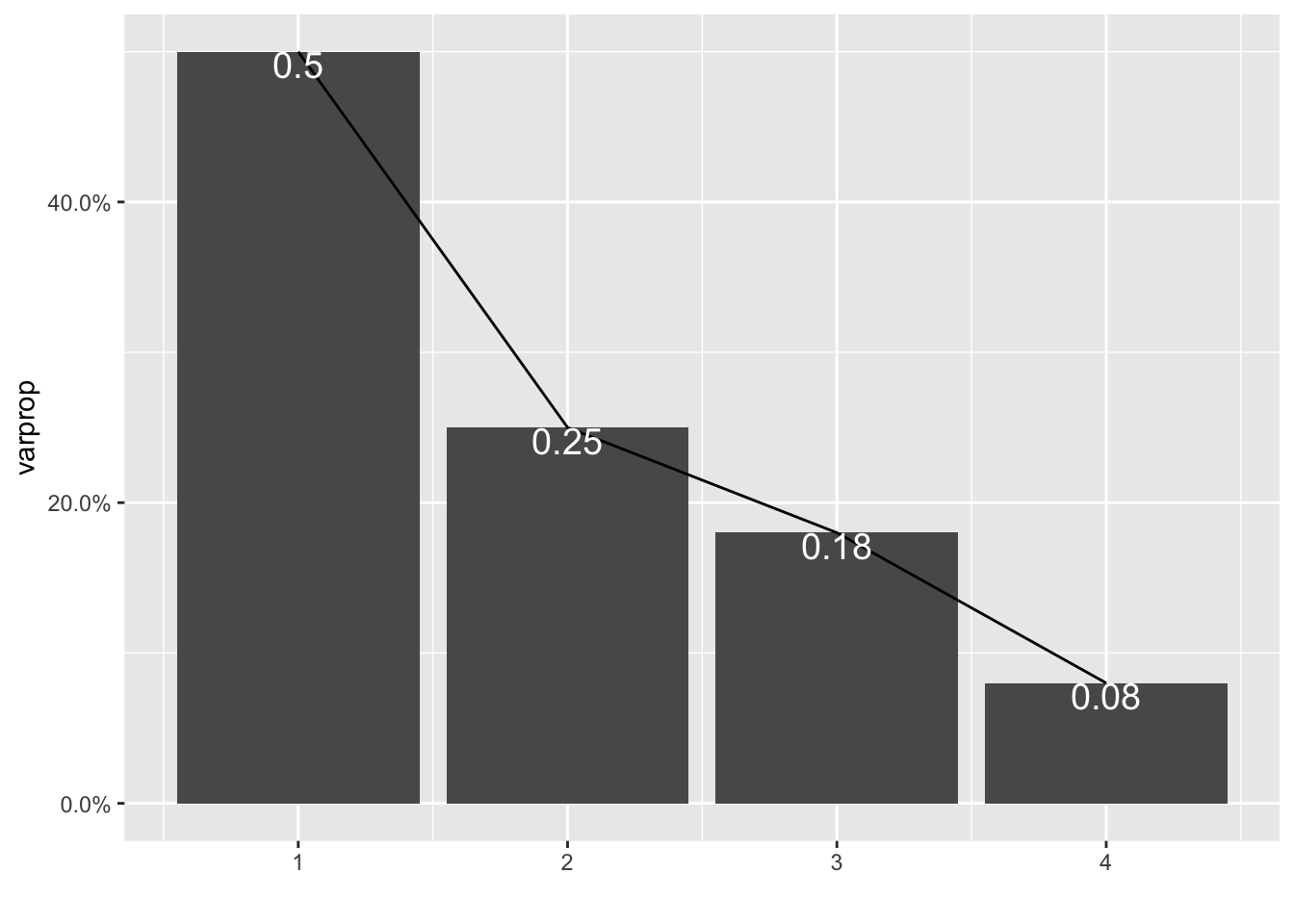
round(cumsum(eigenvals)/sum(eigenvals),2)## [1] 0.50 0.74 0.92 1.00eigenvals## [1] 1.9902039 0.9837192 0.7091042 0.3169727fulldatadf<-data.frame(PC1=f_pca$rotation[4], PC2=f_pca$rotation[1,])
ggplot(fulldatadf, aes(PC1, PC2)) + geom_point()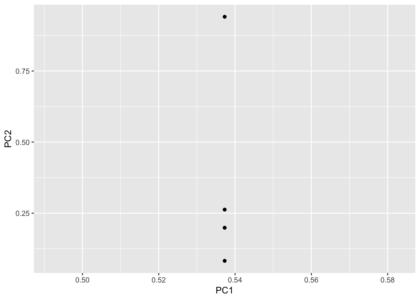
 fviz_pca_var(f_pca,
         col.var = "contrib",
         gradient.cols = c("#00AFBB", "#E7B800", "#FC4E07"),
          repel = TRUE) + ggtitle("PCA Plot")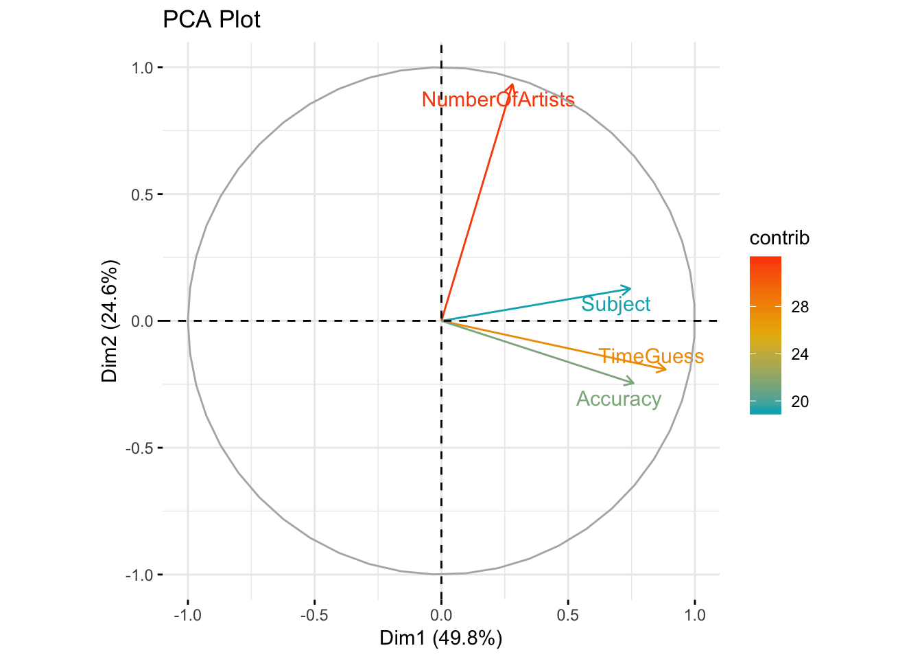
fviz_pca_biplot(f_pca,col.ind = fulldata$Race1)+coord_fixed()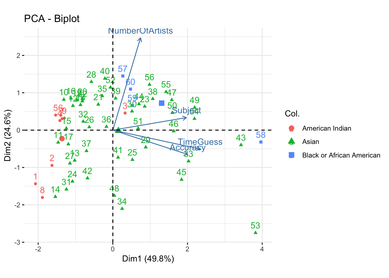
The above biplot graph depicts the principal component analysis of the variables ‘Subject’, ‘TimeGuess’,‘Accuracy’ and ‘NumberOfArtists’. It can be seen that there is a correlation based on the way the two datasets were joined together. The order of the observations dicated the outcome of this particular PCA biplot. The correlation between the variables ‘Subject’, ‘TimeGuess’ and ‘Accuracy’ were the ones that PC2 separated due to them being apart of the ‘MusicTime’ study. Overall, the significance of this biplot is not apparant due to these two datasets being completely different.